The goal of disasteraidr is to have an easy way to download cleaned data
in R from various sources associated with disaster aid allocation in the
UNITED STATES. This is an ongoing project with the University of
Maryland Hazards and Infrastructures team. Currently ‘cleaned’ datasets
come from HUD, NOAA, and FEMA. The main transformations come in CPI
adjustments and conversion of row details associated with the location
to FIPS/county level resolution. US Territories are left out in some of
the dataset such as Guam, Puerto Rico.
Installation
You can install the development version of disasteraidr from Github with:
This is a basic example which shows you how to load in the data:
library(disasteraidr)
# The package currently contains 6 datasets:# These will return <promise> objects. If in R studio, click on# the <promise> tag to load it in.# FEMA Hazard Mitigation Assistance Projects
data("hma")
# NOAA Storm Events
data("noaastorm")
# FEMA Individuals and Household Programs
data("ihp")
# HUD Community Block Grant Program
data("cdbgdr")
# FEMA Public Assistance
data("pa")
# FEMA Disaster Declarations
data("dd")
It produces the quarkus-run.jar file in the target/quarkus-app/ directory.
Be aware that it’s not an über-jar as the dependencies are copied into the target/quarkus-app/lib/ directory.
The application is now runnable using java -jar target/quarkus-app/quarkus-run.jar.
If you want to build an über-jar, execute the following command:
./mvnw package -Dquarkus.package.type=uber-jar
The application, packaged as an über-jar, is now runnable using java -jar target/*-runner.jar.
Creating a native executable
You can create a native executable using:
./mvnw package -Pnative
Or, if you don’t have GraalVM installed, you can run the native executable build in a container using:
MongoDB client (guide): Connect to MongoDB in either imperative or reactive style
RESTEasy Reactive (guide): A JAX-RS implementation utilizing build time processing and Vert.x. This extension is not compatible with the quarkus-resteasy extension, or any of the extensions that depend on it.
A Summernote plugin to enable LaTeX rendering and editing within the Summernote WYSIWYG editor. This plugin integrates MathJax for rendering mathematical expressions, allowing users to include and edit LaTeX code seamlessly.
Features
Add and edit LaTeX equations directly within Summernote.
Render equations with MathJax for accurate mathematical display.
Toolbar integration for easy access to the LaTeX editor.
This project demonstrates Microservice Architecture Pattern using Spring Boot, Spring Cloud, Kubernetes, Istio and gRPC.
It is derived from the MIT-licensed code of Alexander Lukyanchikov, PiggyMetrics.
Functional services
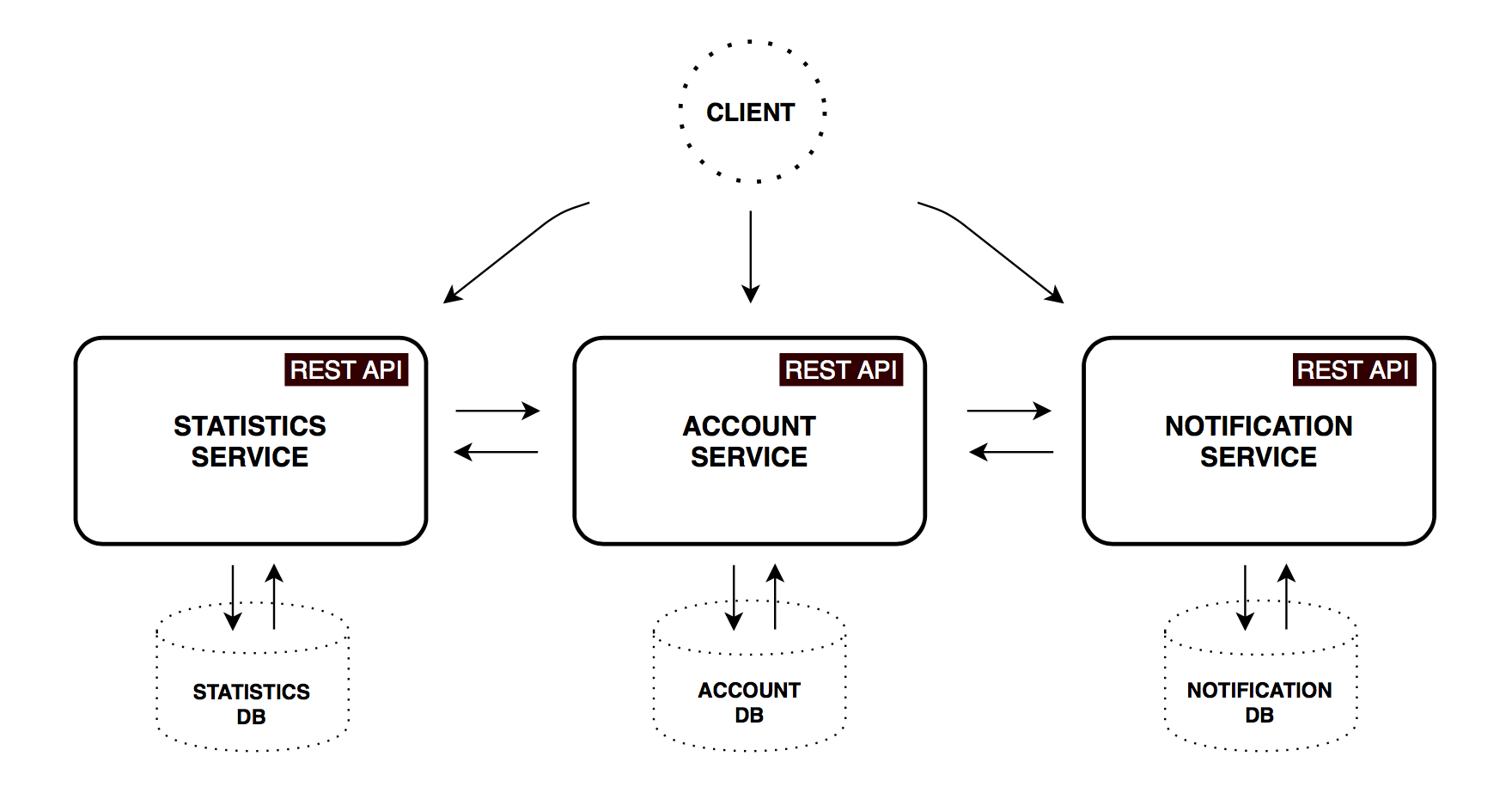
PiggyMetrics was decomposed into three core microservices. All of them are independently deployable applications, organized around certain business domains.
Account service
Contains general user input logic and validation: incomes/expenses items, savings and account settings.
Method
Path
Description
User authenticated
Available from UI
GET
/accounts/{account}
Get specified account data
GET
/accounts/current
Get current account data
×
×
GET
/accounts/demo
Get demo account data (pre-filled incomes/expenses items, etc)
×
PUT
/accounts/current
Save current account data
×
×
POST
/accounts/
Register new account
×
Statistics service
Performs calculations on major statistics parameters and captures time series for each account. Datapoint contains values, normalized to base currency and time period. This data is used to track cash flow dynamics in account lifetime.
Method
Path
Description
User authenticated
Available from UI
GET
/statistics/{account}
Get statistics for the specifed account
GET
/statistics/current
Get statistics for the current account
×
×
GET
/statistics/demo
Get demo account statistics
×
PUT
/statistics/{account}
Create or update time series datapoint for the specified account
Notification service
Stores users contact information and notification settings (like remind and backup frequency). Scheduled worker collects required information from other services and sends e-mail messages to subscribed customers.
Method
Path
Description
User authenticated
Available from UI
GET
/notifications/settings/current
Get current account notification settings
×
×
PUT
/notifications/settings/current
Save current account notification settings
×
×
Notes
Each microservice has it’s own database, so there is no way to bypass API and access persistance data directly.
In this project, I use MongoDB as a primary database for each service. It might also make sense to have a polyglot persistence architecture (сhoose the type of db that is best suited to service requirements).
Service-to-service communication is quite simplified: microservices talking using only synchronous REST API. Common practice in a real-world systems is to use combination of interaction styles. For example, perform synchronous GET request to retrieve data and use asynchronous approach via Message broker for create/update operations in order to decouple services and buffer messages. However, this brings us to the eventual consistency world.
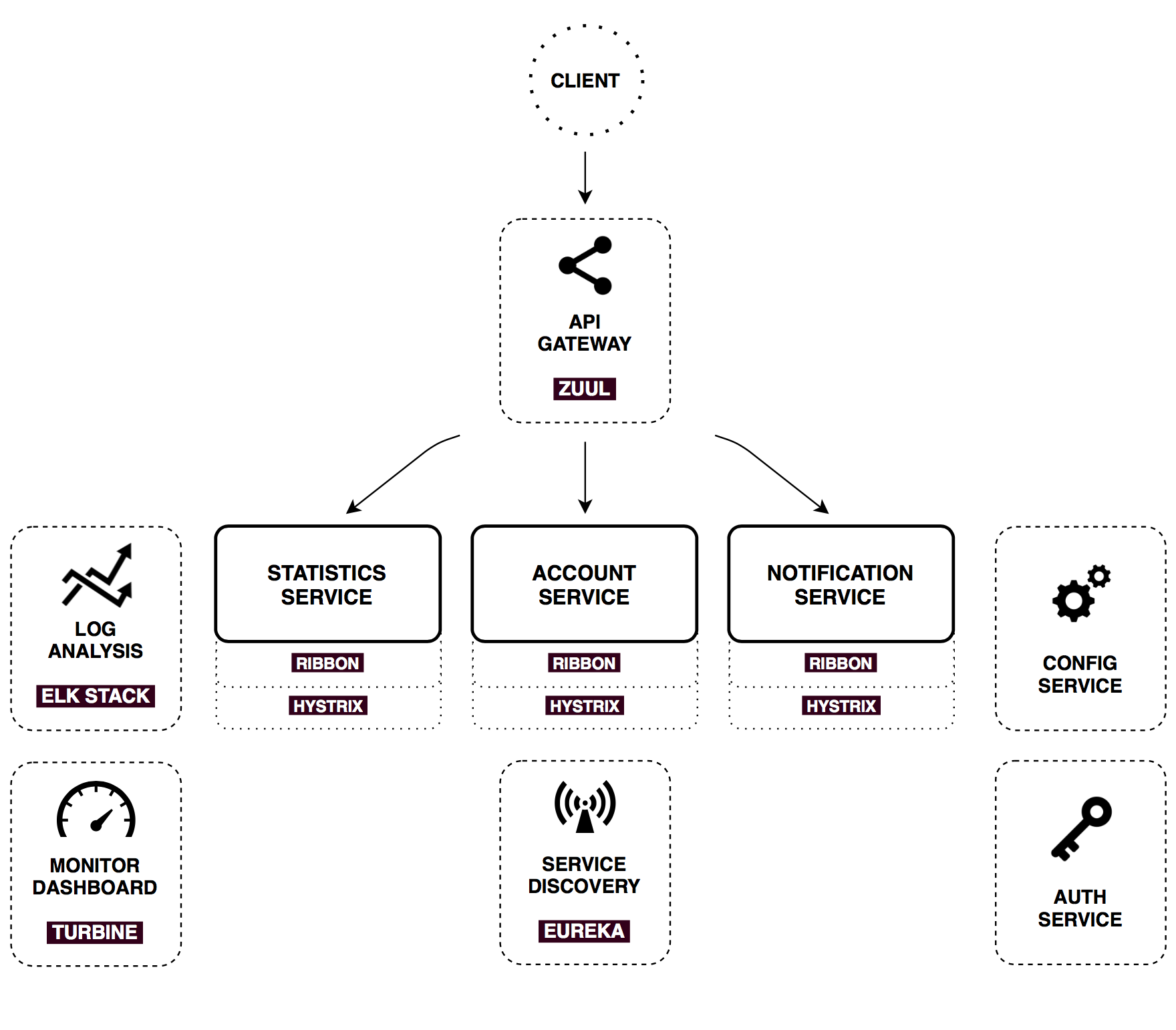
Infrastructure services
There’s a bunch of common patterns in distributed systems, which could help us to make described core services work. Spring cloud provides powerful tools that enhance Spring Boot applications behaviour to implement those patterns. I’ll cover them briefly.
Config service
Spring Cloud Config is horizontally scalable centralized configuration service for distributed systems. It uses a pluggable repository layer that currently supports local storage, Git, and Subversion.
In this project, I use native profile, which simply loads config files from the local classpath. You can see shared directory in Config service resources. Now, when Notification-service requests it’s configuration, Config service responses with shared/notification-service.yml and shared/application.yml (which is shared between all client applications).
Client side usage
Just build Spring Boot application with spring-cloud-starter-config dependency, autoconfiguration will do the rest.
Now you don’t need any embedded properties in your application. Just provide bootstrap.yml with application name and Config service url:
With Spring Cloud Config, you can change app configuration dynamically.
For example, EmailService bean was annotated with @RefreshScope. That means, you can change e-mail text and subject without rebuild and restart Notification service application.
Authorization responsibilities are completely extracted to separate server, which grants OAuth2 tokens for the backend resource services. Auth Server is used for user authorization as well as for secure machine-to-machine communication inside a perimeter.
In this project, I use Password credentials grant type for users authorization (since it’s used only by native PiggyMetrics UI) and Client Credentials grant for microservices authorization.
Spring Cloud Security provides convenient annotations and autoconfiguration to make this really easy to implement from both server and client side. You can learn more about it in documentation and check configuration details in Auth Server code.
From the client side, everything works exactly the same as with traditional session-based authorization. You can retrieve Principal object from request, check user’s roles and other stuff with expression-based access control and @PreAuthorize annotation.
Each client in PiggyMetrics (account-service, statistics-service, notification-service and browser) has a scope: server for backend services, and ui – for the browser. So we can also protect controllers from external access, for example:
As you can see, there are three core services, which expose external API to client. In a real-world systems, this number can grow very quickly as well as whole system complexity. Actually, hundreds of services might be involved in rendering of one complex webpage.
In theory, a client could make requests to each of the microservices directly. But obviously, there are challenges and limitations with this option, like necessity to know all endpoints addresses, perform http request for each peace of information separately, merge the result on a client side. Another problem is non web-friendly protocols which might be used on the backend.
Usually a much better approach is to use API Gateway. It is a single entry point into the system, used to handle requests by routing them to the appropriate backend service or by invoking multiple backend services and aggregating the results. Also, it can be used for authentication, insights, stress and canary testing, service migration, static response handling, active traffic management.
Netflix opensourced such an edge service, and now with Spring Cloud we can enable it with one @EnableZuulProxy annotation. In this project, I use Zuul to store static content (ui application) and to route requests to appropriate microservices. Here’s a simple prefix-based routing configuration for Notification service:
That means all requests starting with /notifications will be routed to Notification service. There is no hardcoded address, as you can see. Zuul uses Service discovery mechanism to locate Notification service instances and also Circuit Breaker and Load Balancer, described below.
Monitor dashboard
In this project configuration, each microservice with Hystrix on board pushes metrics to Turbine via Spring Cloud Bus (with AMQP broker). The Monitoring project is just a small Spring boot application with Turbine and Hystrix Dashboard.
Let’s see our system behavior under load: Account service calls Statistics service and it responses with a vary imitation delay. Response timeout threshold is set to 1 second.
0 ms delay
500 ms delay
800 ms delay
1100 ms delay
Well behaving system. The throughput is about 22 requests/second. Small number of active threads in Statistics service. The median service time is about 50 ms.
The number of active threads is growing. We can see purple number of thread-pool rejections and therefore about 30-40% of errors, but circuit is still closed.
Half-open state: the ratio of failed commands is more than 50%, the circuit breaker kicks in. After sleep window amount of time, the next request is let through.
100 percent of the requests fail. The circuit is now permanently open. Retry after sleep time won’t close circuit again, because the single request is too slow.
Log analysis
Centralized logging can be very useful when attempting to identify problems in a distributed environment. Elasticsearch, Logstash and Kibana stack lets you search and analyze your logs, utilization and network activity data with ease.
Ready-to-go Docker configuration described in my other project.
Security
An advanced security configuration is beyond the scope of this proof-of-concept project. For a more realistic simulation of a real system, consider to use https, JCE keystore to encrypt Microservices passwords and Config server properties content (see documentation for details).
Infrastructure automation
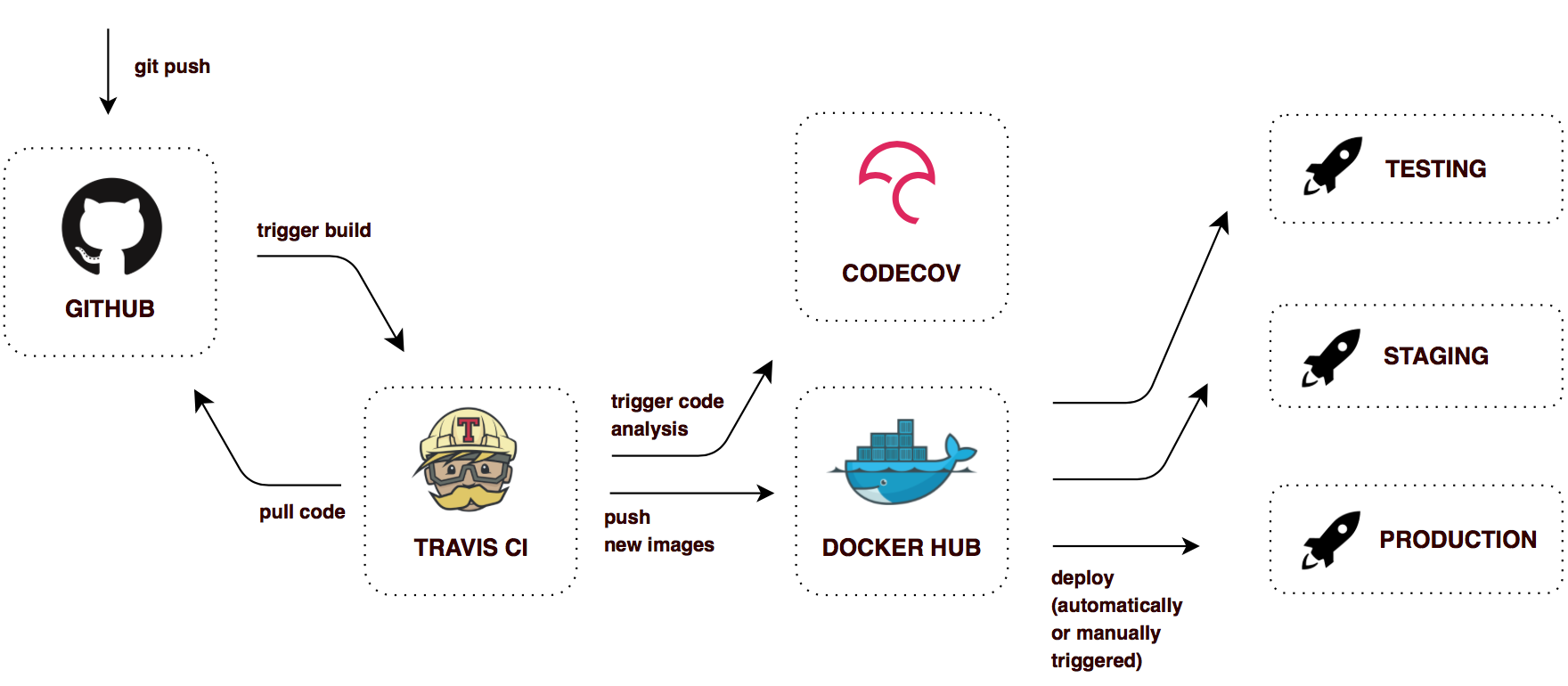
Deploying microservices, with their interdependence, is much more complex process than deploying monolithic application. It is important to have fully automated infrastructure. We can achieve following benefits with Continuous Delivery approach:
The ability to release software anytime
Any build could end up being a release
Build artifacts once – deploy as needed
Here is a simple Continuous Delivery workflow, implemented in this project:
In this configuration, Travis CI builds tagged images for each successful git push. So, there are always latest image for each microservice on Docker Hub and older images, tagged with git commit hash. It’s easy to deploy any of them and quickly rollback, if needed.
How to run all the things?
Keep in mind, that you are going to start 8 Spring Boot applications, 4 MongoDB instances and RabbitMq. Make sure you have 4 Gb RAM available on your machine. You can always run just vital services though: Gateway, Registry, Config, Auth Service and Account Service.
and set its policy value to disabled. This disables automatic sidecar injection unless the pod template spec contains
the sidecar.istio.io/inject annotation with value true.
Add the bitnami and codecentric Helm repositories:
Deploy PostgreSQL, Apache Kafka and Keycloak to Kubernetes:
helm install charts/pgm-dependencies
Production mode
In this mode, Kubernetes pods will be created using the latest images from Docker Hub. Just run
helm install charts/piggymetrics
Make sure all microservices runs. The command
kubectl get pods
should return something like:
and then go to http://localhost.
Development mode
If you’d like to build images yourself (with some changes in the code, for example), first install Skaffold.
To build and deployed all microservices to Kubernetes run skaffold dev.
SV callers like lumpy look at split-reads and pair distances to find structural variants.
This tool is a fast way to add depth information to those calls. This can be used as additional
information for filtering variants; for example we will be skeptical of deletion calls that
do not have lower than average coverage compared to regions with similar gc-content.
In addition, duphold will annotate the SV vcf with information from a SNP/Indel VCF. For example, we will not
believe a large deletion that has many heterozygote SNP calls.
duphold takes a bam/cram, a VCF/BCF of SV calls, and a fasta reference and it updates the FORMAT field for a
single sample with:
DHFC: fold-change for the variant depth relative to the rest of the chromosome the variant was found on
DHBFC: fold-change for the variant depth relative to bins in the genome with similar GC-content.
DHFFC: fold-change for the variant depth relative to Flanking regions.
It also adds GCF to the INFO field indicating the fraction of G or C bases in the variant.
After annotating with duphold, a sensible way to filter to high-quality variants is:
In our evaluations, DHFFC works best for deletions and DHBFC works slightly better for duplications.
For genomes/samples with more variable coverage, DHFFC should be the most reliable.
SNP/Indel annotation
NOTE it is strongly recommended to use BCF for the --snp argument as otherwise VCF parsing will be a bottleneck.
A DEL call with many HETs is unlikely to be valid.
When the user specifies a --snp VCF, duphold finds the appropriate sample in that file and extracts high (> 20) quality, bi-allelic
SNP calls and for each SV, it reports the number of hom-refs, heterozygote, hom-alt, unknown, and low-quality snp calls
in the region of the event. This information is stored in 5 integers in DHGT.
When a SNP/Indel VCF/BCF is given, duphold will annotate each DEL/DUP call with:
DHGT: counts of [0] Hom-ref, [1] Het, [2] Homalt, [3] Unknown, [4] low-quality variants in the event.
A heterozygous deletion may have more hom-alt SNP calls. A homozygous deletion may have only unknown or
low-quality SNP calls.
In practice, this has had limited benefit for us. The depth changes are more informative.
Performance
Speed
duphold runtime depends almost entirely on how long it takes to parse the BAM/CRAM files; it is relatively independent of the number of variants evaluated. It will also run quite a bit faster on CRAM than on BAM. It can be < 20 minutes of CPU time for a 30X CRAM.
Accuracy
Evaluting on the genome in a bottle truthset for DEL calls larger than 300 bp:
method
FDR
FN
FP
TP-call
precision
recall
recall-%
FP-%
unfiltered
0.054
276
86
1496
0.946
0.844
100.000
100.000
DHBFC < 0.7
0.018
298
27
1474
0.982
0.832
98.529
31.395
DHFFC < 0.7
0.021
289
32
1483
0.979
0.837
99.131
37.209
Note that filtering on DHFFC < 0.7retains 99.1% of true positives and removes 62.8% (100 – 37.2) of false positives
This was generated using truvari.py with the command:
Note that filtering on DHFFC < 0.7retains 98.5% of DEL calls that are also in the truth-set (TPs) and
removes 84.2% (100 – 15.8) of calls not in the truth-set (FPs)
The truvari.py command used for this is the same as above except for: -s 1000 -S 970
--snp can be a multi-sample VCF/BCF. duphold will be much faster with a BCF, especially if
the snp/indel file contains many (>20 or so) samples.
the threads are decompression threads so increasing up to about 4 works.
Full usage is available with duphold -h
duphold runs on a single-sample, but you can install smoove and run smoove duphold
to parallelize across many samples.
Examples
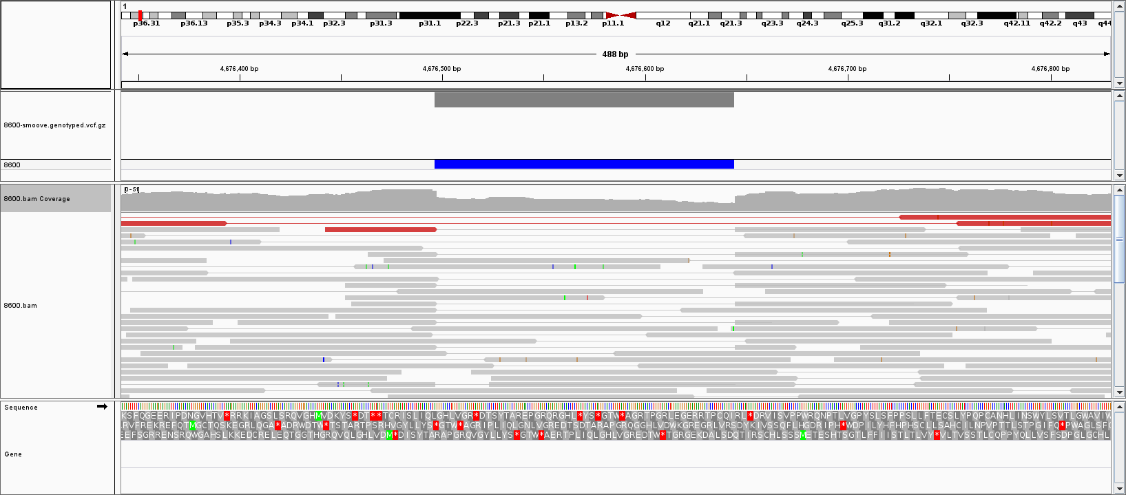
Duplication
Here is a duplication with clear change in depth (DHBFC)
duphold annotated this with
DHBFC: 1.79
where together these indicate rapid (DUP-like) change in depth at the break-points and a coverage that 1.79 times higher than the mean for the genome–again indicative of a DUP. Together, these recapitulate (or anticipate) what we see on visual inspection.
Deletion
A clear deletion will have rapid drop in depth at the left and increase in depth at the right and a lower mean coverage.
duphold annotated this with:
DHBFC: 0.6
These indicate that both break-points are consistent with a deletion and that the coverage is ~60% of expected. So this is a clear deletion.
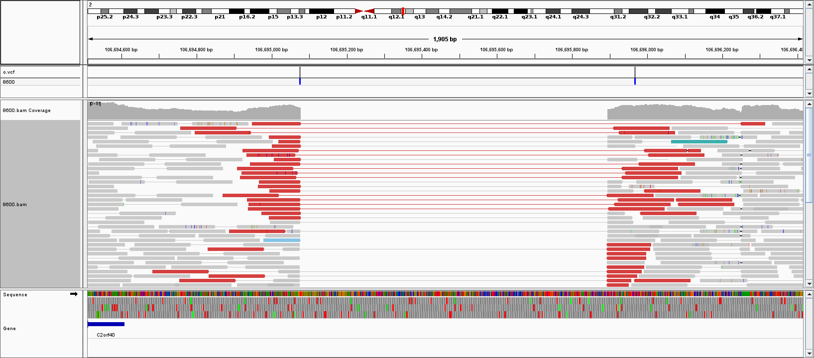
BND
when lumpy decides that a cluster of evidence does not match a DUP or DEL or INV, it creates a BND with 2 lines in the VCF. Sometimes these
are actual deletions. For example:
shows where a deletion is bounded by 2 BND calls. duphold annotates this with:
DHBFC: 0.01
indicating a homozygous deletion with clear break-points.
Tuning and Env vars
The default flank is 1000 bases. If the environment variable DUPHOLD_FLANK is set to an integer, that
can be used instead. In our experiments, this value should be large enough that duphold can get a good estimate
of depth, but small enough that it is unlikely to extend into an unmapped region or another event.
This may be lowered for genomes with poor assemblies.
If the sample name in your bam does not match the one in the VCF (tisk, tisk). You can use DUPHOLD_SAMPLE_NAME
environment variable to set the name to use.
Acknowledgements
I stole the idea of annotating SVs with depth-change from Ira Hall.
Our project will analyze New York City mayoral elections.
We will determine whether there exists a relationship between the quantity of campaign finance donations and electoral results, and whether a donation sum from a particular occupation or industry is likewise related.
Questions
How much financial data play a role in Mayor candidate election outcome.
A Pyspark data parser on Google Colab to edit data into database entry format.
An Amazon Relational Database Service to host a PostgreSQL instance which will serve as a data repository, and a start and end point for the machine learning model.
Supervised categorical machine learning approach using TensorFlow which predicts election outcomes on categorical column attributes.
Dashboard composition with Tableau and Plotly composed with distribution of data, outliers, trends, hypotheses, predictions and conclusions.
Dashboard
Tools used:
Tableau Public
Tableau Javascipt API
Description:
We have built our visualizations using Tableau. Also, we have built our website using the Tableau JavaScript API, and have hosted it on Github.
Anyone who is interested in learning about the role finance has on New York City’s mayoral elections. They can see the difference between contributions and expenditures between candidates, as well as their significance.
What are our vizualizations going to tell us?
We have tried to visually understand how some of the data variables differ for a given candidate, such as ZIP codes, quarters (of a year), number and total amount of contributions, and total amount of expenditures per election year.
We have contributions and expenditures received and spent for each participating candidate. The range we have chosen is between 2001 and 2021 (the general election for the latter has yet to take place,) inclusive.
How do we add interactive elements to our dashboard?
We have added filters to our dashboard, making them available via the All Using Related Data Sources option, so that any selection through the filter applies to all worksheets that are in any way related to the data source.
Please note that we have used multiple data sources and have used the Edit Blend Relationships option to link primary and secondary data sources.
We have added Highlight Actions to our dashboard which work when a user hovers over the source sheets.
We have added interactive text to our dashboard which dynamically change the text based on which election year was selected.
Features
We have a container in which each of the dashboards appear after clicking either the Previous or Next buttons.
Upon entering the homepage, one is taken to the first dashboard, so the Previous button is disabled.
The Next button takes the user from the first dashboard to the next, and is then disabled once the user reaches the last dashboard. The user can always click on the Home button to return to the homepage.
There is a graph that shows how many contributions came in for each of the candidates. Here, the candidate name can be selected to see data changes in the map and quarterly contribution graphs.
The map is color-coded to better identify which zip codes had higher contributions.
Our visualization shows the top candidates sorted by the amount received and spent. Highlight Hover action has been created on this page to enhance visual effects.
Data
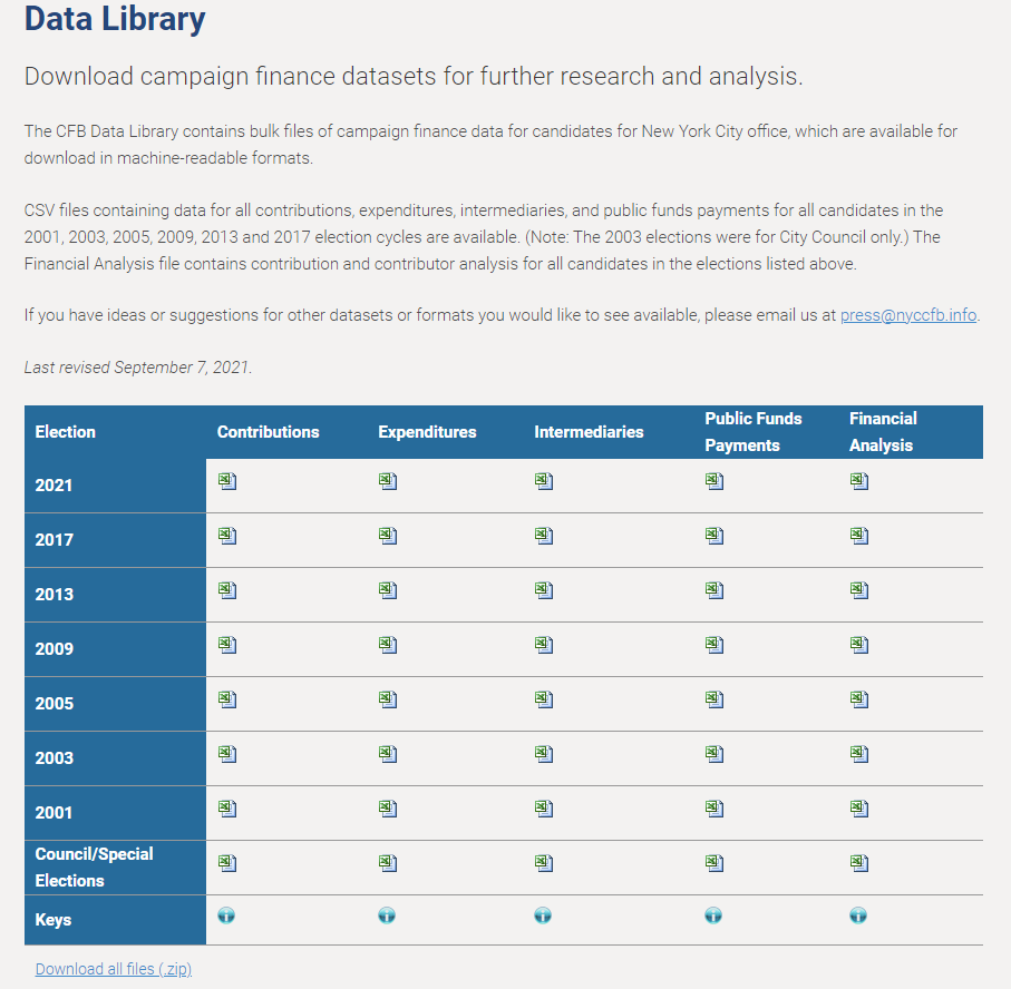
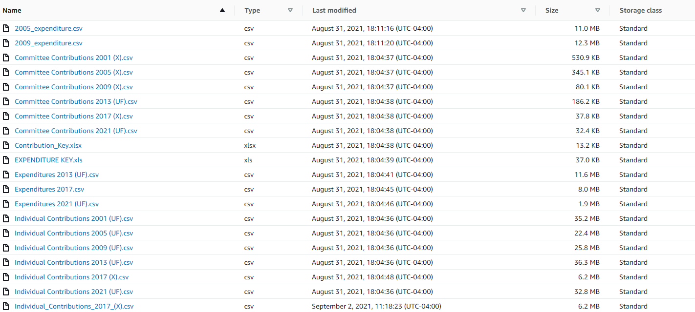
The data we obtained for this project include publicly available records for each NYC mayoral election campaign donation reports from Individuals and Committee/Organizations. The following records also included the Expenditure spending per election year that were tracked by each candidate. We were able to gather the data reports for the six most recent election terms, namely for 2001, 2005, 2009, 2013, 2017, and 2021.
The following data that was obtained from the New York City Campaign Finance Board contained three separate .csv files for each election year: Individual, Committee and Expenditure reports.
The Individual Donation reports contained data that was tracked based on an individual’s donation contribution to a particular candidate. Each row highlights the donation amount, the donor’s State, City, and Zip Code and the date each transaction was made. The following transactions contained an estimated amount of 65,000 records of tracked donations per election year.
The Committee Donation reports were similar to the Individual Donation reports. The main difference was that the donations were tracked based on larger Corporation, Labor Union, Organizations, LLC, Political Action Committees, and Party Committees donations to the candidate. The following tracked Committee Donations per election year contained an average amount of 300-500 donation records per election.
The Expenditure report tracked each participating candidate’s per election year expenditure spending during their campaigning. Some highlighted records that were tracked are Television and Radio advertisements, Professional Services, Campaign Worker Salaries, Polling Costs, and many others. The following expenditure transactions were tracked by the location of the transaction that included the amount, date of transaction, City, State, and Zip Codes. The Expenditure reports contained an average amount of 12,000 tracked transactions per election year.
Please see the following screen shot that shows the home page of where we have obatined all of our data.
ETL Process
The steps taken to extract, transform, and load the data for analysis are as follows:
• From the New York City Campaign Finance Board webpage download the previous six election years from 2001,2003,2005,2009,2013,2017, and 2021 data sets that contain individual donation data and committee donation data per election year as local CSVs.
• Also extract the previous six election years for each candidate’s expenditures as separate data sets from the New York City Campaign Finance Board.
• Study each of the 18 Excel data sets and determine which columns hold value for our final outcome. (All Raw CSVs can be found within Resources > Raw CSVs Folder)
• Create a RDS and S3 within Amazon Web Services to store the following data sets and share publicly with team.
• Upload each election year CSV for individual donations, committee donations, and candidate expenditures within Google Colab.(The following files can be found within Resources > Contribution tables (CSVs) and Expenditure Reports (CSVs))
• Perform Pyspark functions of reading CSVs in data frames, dropping columns, changing data types, changing column names, converting the value names within each column, filter the data frames to display only the mayor elections and participants within the mayor election year, create a total sum column that’s added by the donation amount, candidate match amount, and previous donation amount (The following scripts can be found within DataCleaningAndTransforming > Google Colab Documents)
• Once the data frame is reviewed and approved by the team export the clean data frame into a new CSV (Transformed dataframes into new CSVs can be found in Resources )
• Export and bridge the clean data frame tables for each election year to connect with the RDS server and Postgres SQL.
• Create the join on committees and individual tables to prepare for machine learning.
• Merge/Union the tables by the individual data frame, committe contribution data frame, as well as the expenditure report dataframes all as a single CSV per year. (The following merged tables can be found here Resources > Merged Contribution and Expenditure (CSVs))
• Determining columns necessary for ML
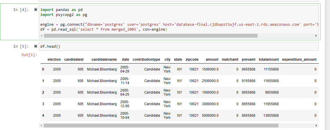
•Connect PGAdmin with Pandas to read in 2021,2017,2013,2009,2005, and 2001 merged files to begin Machine Learning.
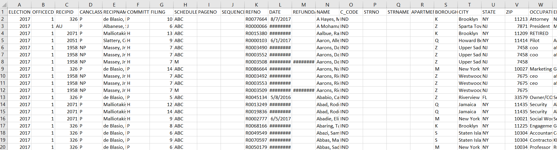
Pre ETL of the raw campaign data
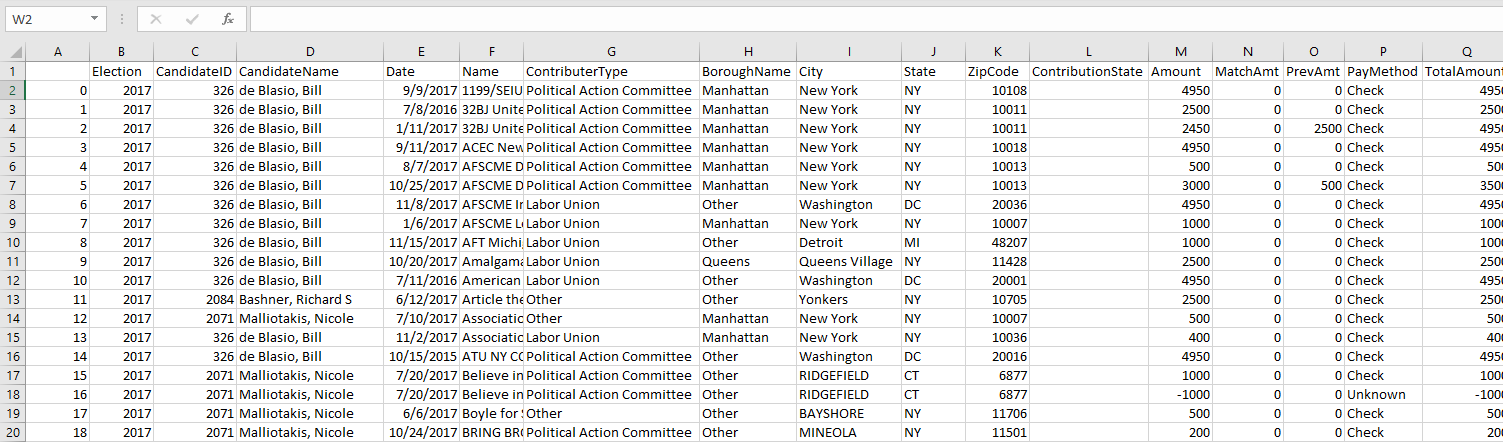
Post ETL of the cleaned campaign data
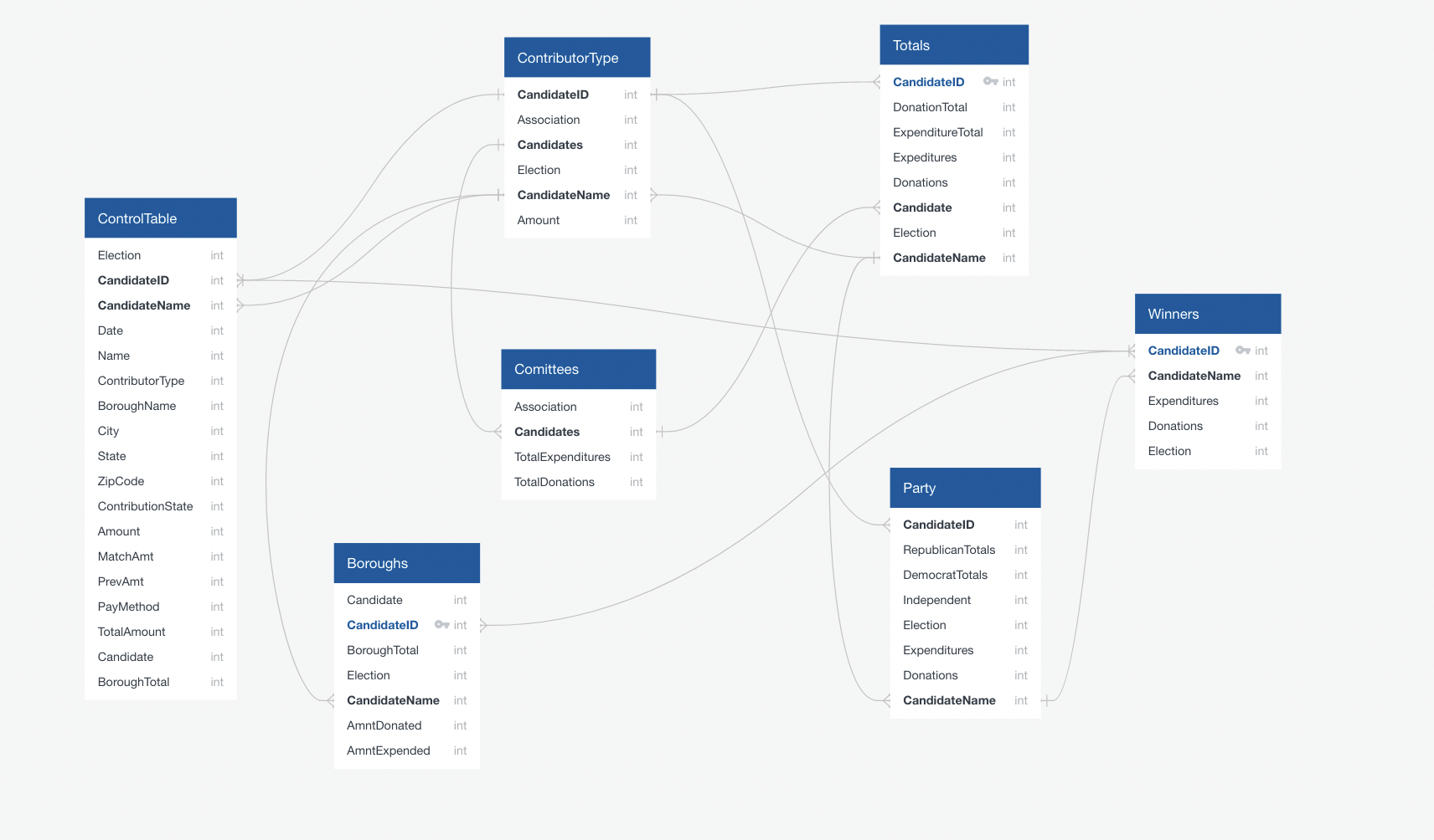
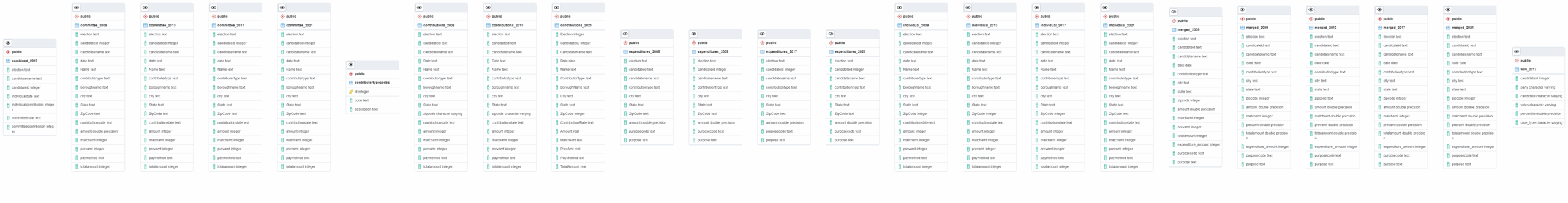
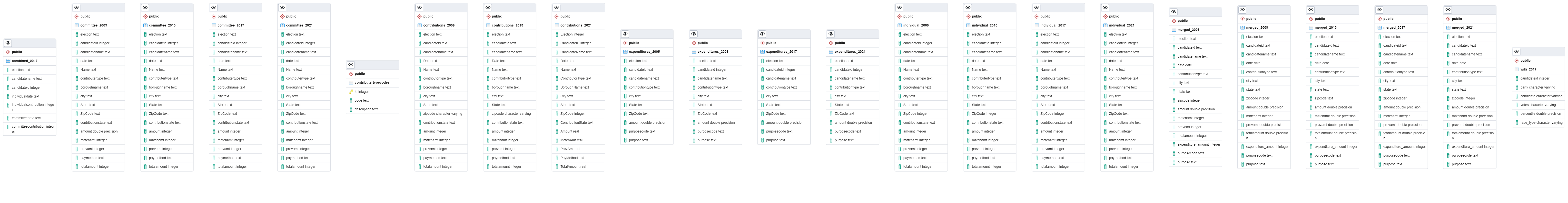
ERD OUTLINE
ERD CURRENT TABLES
ML Model
Overview
The purpose of our model is to create a supervised learning algorithm to predict the total amount of money raised in a particular zip code for every New York City Mayoral election between 2005 and 2021. For our model, we used a Random Forest Regressor. The code for our data can be found within the MLScripts folder of our repository. The models are named Regressions_2005, Regressions_2009, Regressions_2013, Regressions_2017, and Regressions_2021, with the numbers at the end corresponding with the election year.
Preprocessing
Feature Engineering
The CSV files were initially sourced from the NYC Campaign Finance Board’s website which were first cleaned using SQL and PgAdmin and were then loaded onto a notebook. The raw CSV files contained columns with the the amount, matched amount, and previous contributions, and we then aggregated those three columns to create a new column with the total amount of contributions given to a particular candidate. We then used Pandas’ groupby function to groupby the sum of total amount of contribution based on the zip code from where the donation originated.
Feature Selection
To determine which features we deemed were necessary to test our model, we created various graphs of our raw data to determine whether we could visually identify a relationship between the total amount of money raised and a particular zip code. Using a the Pandas groupby function and matplotlib, we created bar charts which indicated a relationship between the total amount raised and particular zip codes. Initially, the goal of our project was to create a supervised classification model which could determine the outcome of past elections using these same features but we determined such a model would not be feasible in the allotted time, therefore we shifted to the current regression model. However, during our feature selection process we determined that the same features would be applicable to both models. Two columns of the initial CSV were removed prior to being fed into the model as we determined that they added no value to the model. These were the year of election column and the previous amount column. The former was removed because it was a superfluous column that added no value while the latter was removed because the data from that column was already factored in the amount column. The final features selected for our models are as follows:
Zip code
Type of contribution (individual, corporation, PAC, et al.)
Date of contribution
City of contribution
State of contribution
Amount of contribution
Amount of contribution matched by the city
The amount of money spent by the candidate’s campaign (expenditures)
Encoding
To encode our data we used sklearn’s label encoder. We encoded all non-numerical data within our dataset with sklearn’s fit_transform function to ensure our model would be able to read it. We did not encode the amount, matched amount, expenditures, and total amount, as we needed them unencoded to be able to visually analyze our data and there did not seem to be any major effects to our model without such encoding.
Model Choice
We used a Random Forest Regressor for our model. We chose this model for a variety of reasons, which are as follows:
Able to work around outliers
The training and prediction speeds are quick
Contains low bias and moderate variance
It is capable of handling unbalanced data
The model is not without it’s drawbacks, as it can be difficult to interpret, it can often overfit the data, and can take up a lot of memory if the dataset is large.
Initially, we were using the Random Forest Classifier for our model as we were attempting to create a classification model which can predict the outcomes of an election but we decided that a regression model to predict the total amount of money raised would be more realistic to complete in the allotted time. We therefore decided to change our model to the current one.
Training and testing
We trained and tested our dataset using sklearn’s train_test_split. The features listed above were all used as the X values and the total amount raised was used as the y value. The training size was 0.7 and testing size was 0.3 which was determined after various test models suggested this was the optimal split. The data was then fitted and tested using the Random Forest Regressor, after which the predictions were generated.
Accuracy Score
To test for accuracy, we applied the R-squared and the Root-mean-square deviation error (RMSE) functions to our predictions. As we tested the model on four datasets, the R-squared values are as follows:
2005: 0.72
2009: 0.92
2013: 0.85
2017: 0.92
2021: 0.85
The Root-mean-square deviation values are as follows:
2005: 0.009
2009: 0.004
2013: 0.014
2017: 0.013
2021: 0.008
These high correlation results indicates that there is a correlation between the features we selected for our model and the the total amount of money raised in a particular zip code. The rather high correlation calculated by our model can also indicate that there were bugs in our code that led to some kind of imbalance that skewed our data. The values for the RMSE deviations tell us that there is a low difference between the test and predicted values, indicating that there is indeed a relationship between our features and the total amount raised, however there is a possibility that errors occurred during the construction of the code that may have led to some form of data leakage and therefore skewing the results. Further analyses must be done before we can use these as conclusive results.
We have the datasets which we will be using for our project. Refer to https://www.nyccfb.info/follow-the-money/cunymap-2021 in order to look at the individual and committee level contributions to our Mayor Candidates.
Refer to 2017_Mayor_IC.csv and 2017_Mayor_CC.csv files in our repository for sample data.
At first we had decided to get data from Legistar API provided by NYC Coucil website. We were successfully able to read data from the API. Refer to LegistarAPI.ipynb file posted on https://github.com/ssheggrud/Mod_20_Project/tree/05_Pooja . Altough we later decided that had we used that data, it would have unnecessarily added complexity to our code. Hence, we decided to add each years election results manually to a manually sourced excel as as individual column. We will name this column “Won/Elected”.
We have come up with few dashboards and a storyboard in Tableau.
We have started work on linking our tableau vizualization to our html page using Tableau Javascript API.
Successful transformed the 2017 Election year Individual, Committee, and Expenditures raw CSV’s into a transformed and test ready file from Google Colab using Pyspark and Pandas while exporting the cleaned dataframes into SQL and new local CSVs. To see the final 2017 transformation process please refer to the DataCleaningTransformation folder.
Static table, join script and other DB scripts were added to the DBScripts folder.
A base sklearn’s K-nearest neighbor model can been created and run on a sample 2017 data.
Week 3:
Tweaking the website to best display the Tableau data. HTML and CSS files were edited to better display the API from Tableau.
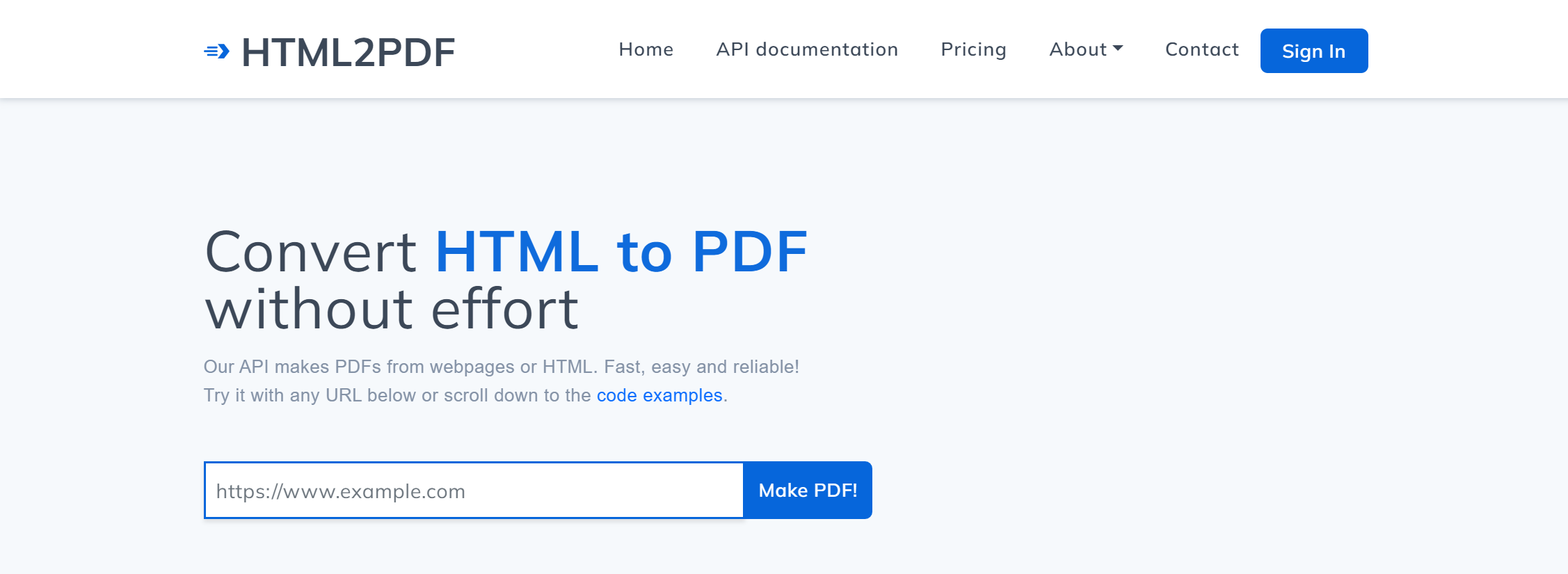
This list aims to be the ultimate list of HTML to PDF APIs. We have curated this list of the best HTML to PDF APIs based on their ease of use, documentation, and pricing. We also use the community votes from APIFinder for the ranking.
Comparing the Pricing
Some APIs are charging based on the amount of PDFs created while others are also charing based on the size of the PDF that has been created. When an API is charging based on the size of the PDF, we have calculated the price based on a PDF of 2MB in size. We feel like thats a reasonable size for the average PDF.
Collaboration
If you have any suggestions or spot any mistakes, please let us know by creating an issue or pull request.
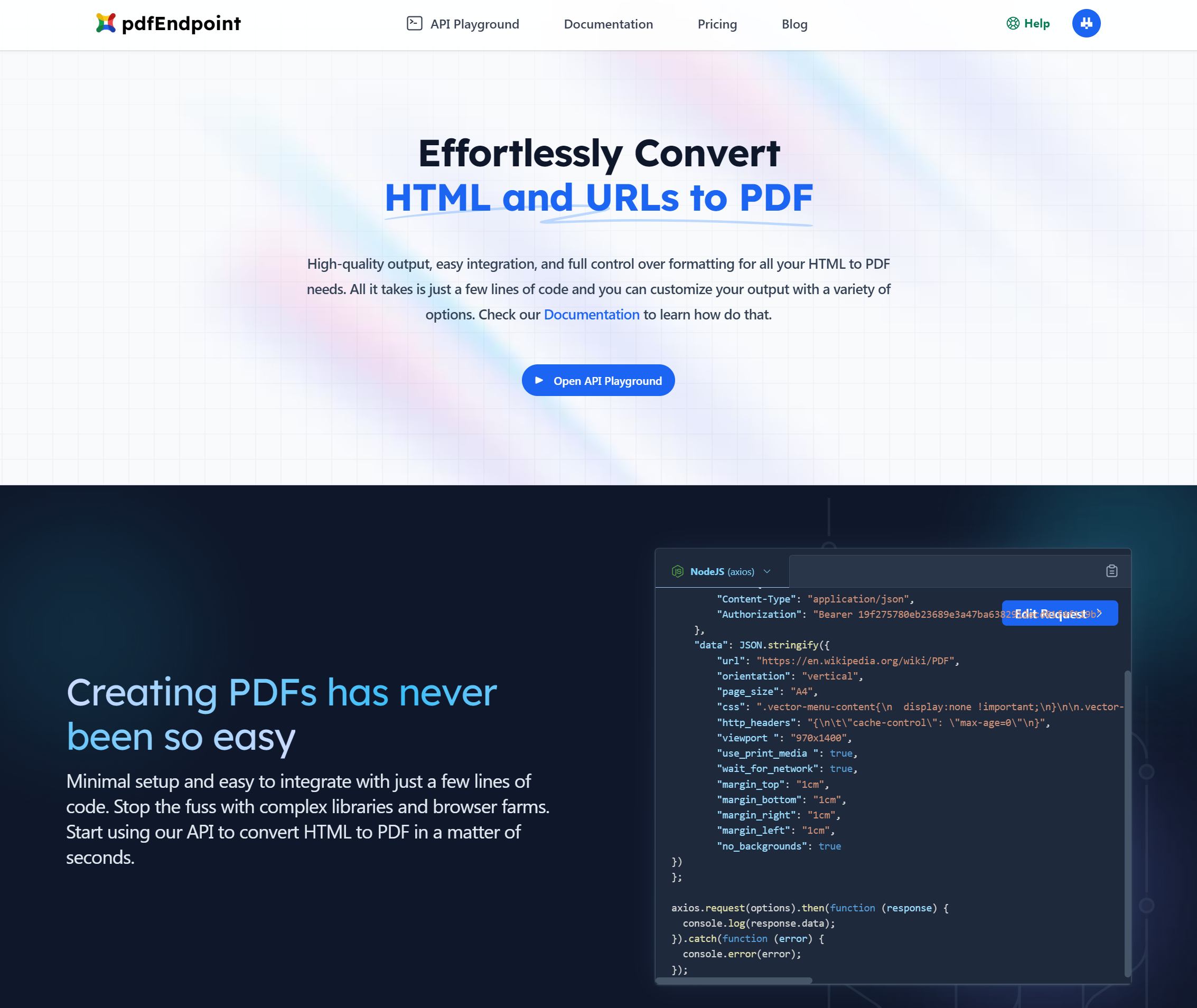
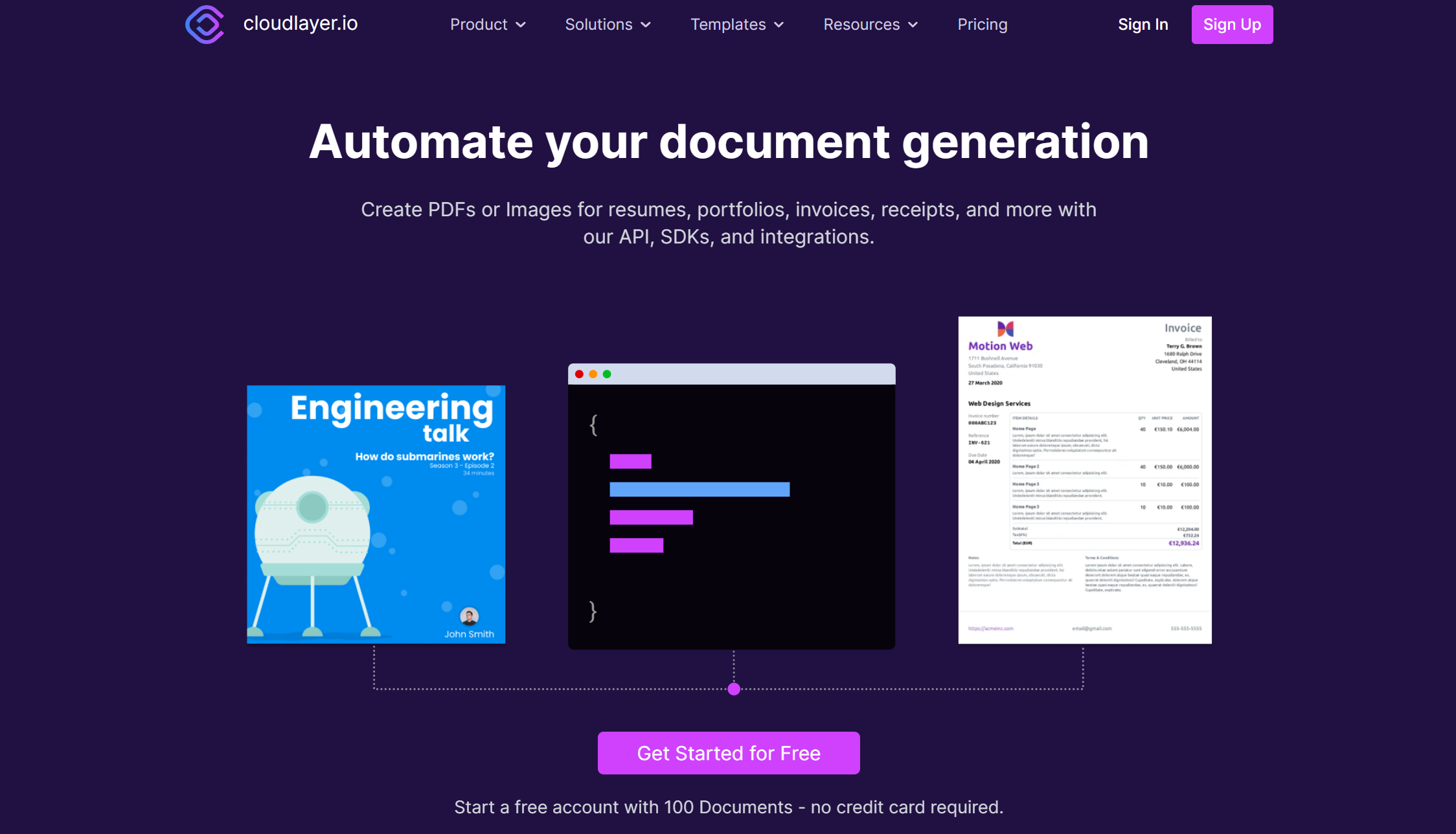
The playground allows you to test the API without having to sign up for free. We think this is the best playground in this list so be sure to give it a try!
Pricing is based on the number of PDFs you generate per month with no file size limit. You can generate an unlimited number of PDFs per month since all plans have the option for overusage so you do not get limited if you have reached your monthly quota.
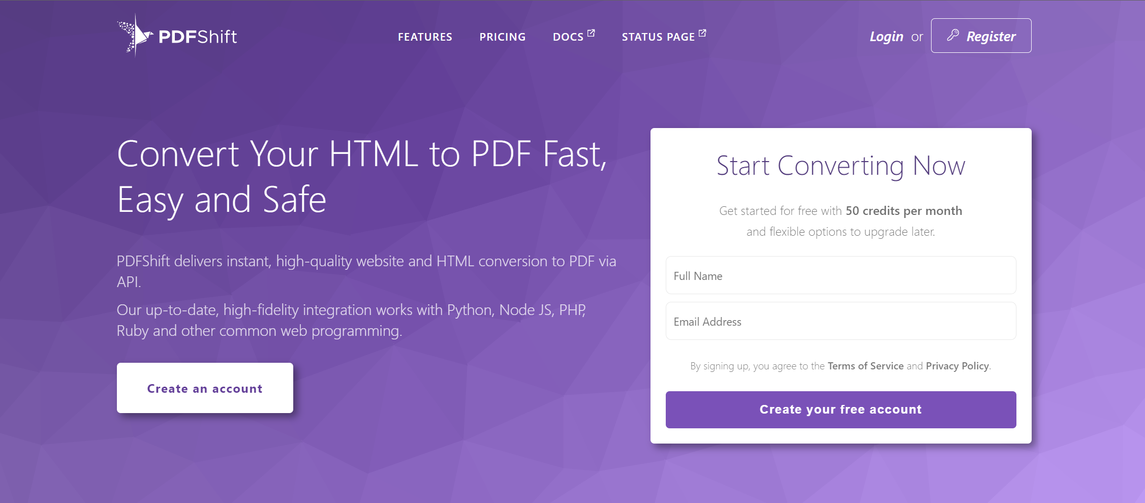
Pricing: Monthly Subscription – 1MB per credit – Pricing Page
PDFShift is charging based on credits per created PDF and the size of the PDF. A PDF of 1MB will be charged as 1 credit.
Rate Limit: 240 requests per minute
Maintainer Remarks:
The Owner/Developer of PDFShift is publishing his revenue on IndieHackers. This is a great way to see if the serviece your are using is going to be around for longer. It also shows that the owner is very transparent and honest about his business.
Rate Limit: Free Plan – 2 requests per minute / Paid Plan – 45 requests per minute
Maintainer Remarks:
⚠️ The basic plan does not support https. So your requests will not be encrypted. This is a big security risk so make sure you know what you are doing.
Rate Limit: 15 requests per minute / up to 360 requests per minute
Maintainer Remarks:
Weird pricing based on subscriptions, licenses and credits. I did not quite understand the pricing when checking the page but your mileage may vary ( or you are smarter then me 🙂 ).
SelectPDF is the only API in this list that offers an unlimited plan. This is a great option if you need to convert a lot of documents. Additionaly you can purchase standalone licenses for your server.
Rate Limit: NOT PROVIDED
Maintainer Remarks:
While SelectPDF does offer an unlimited plan we could not find any information on what the rate limits are or how many concurrent requests are allowed. You might want to reach out to their support before using the unlimited plan since the rate limit could be very low.
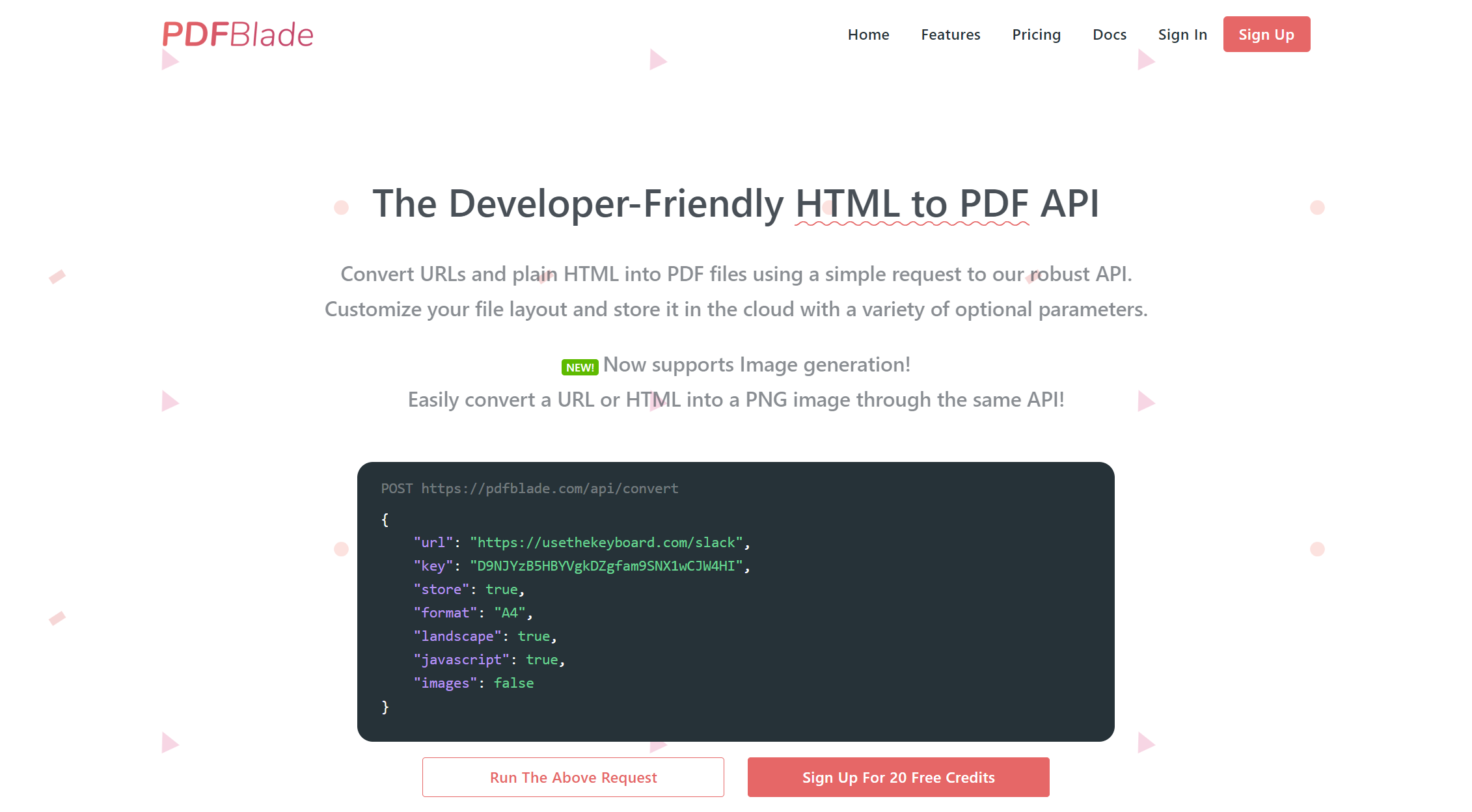
PDFBlade is billied using a credit based system. Credits can be purchased in packages starting at 20 credits for $1.00. The price per credit decreases with the amount of credits you purchase. The more credits you purchase the cheaper they get. Credits roll over to the next month if you do not use them up.
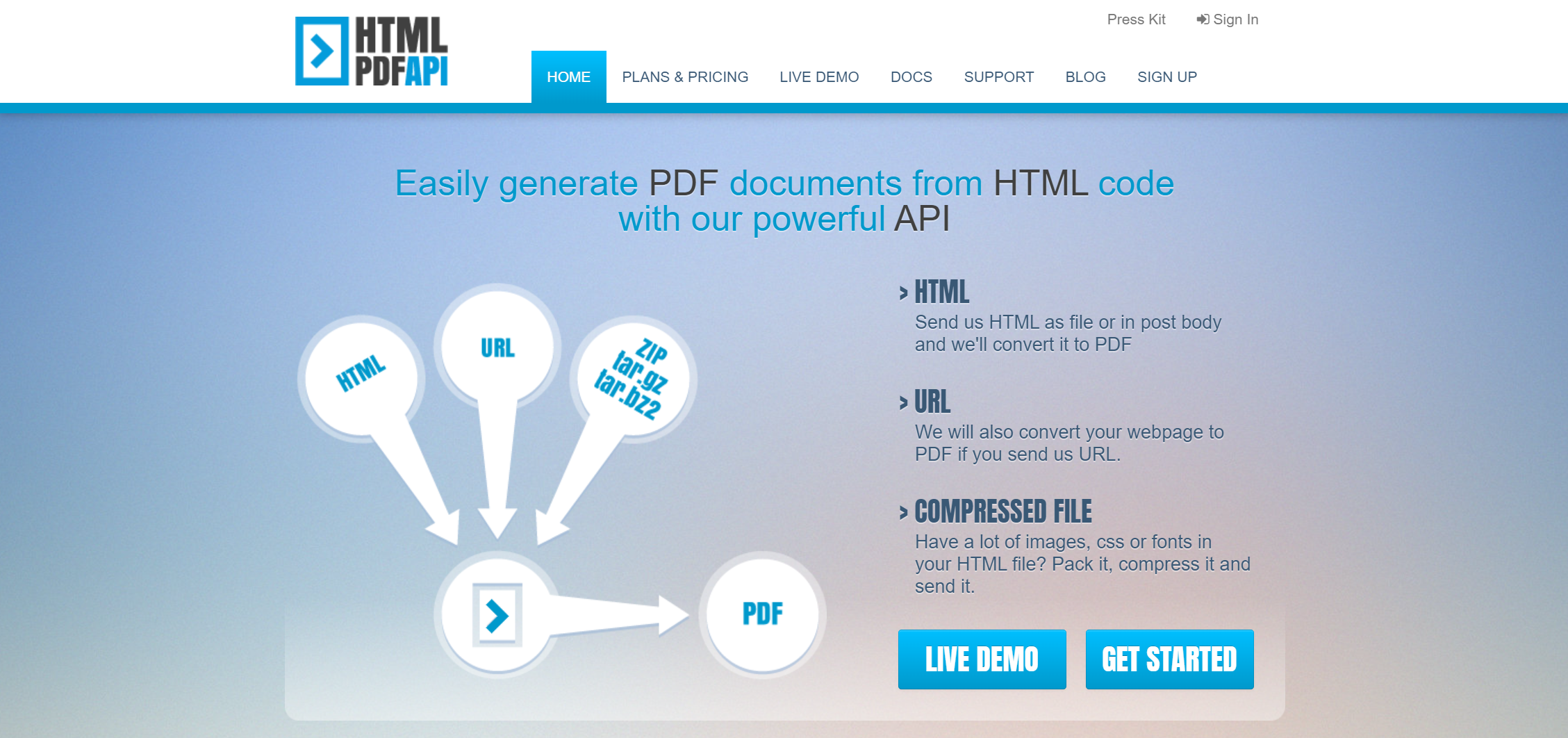
HTMLPDFAPI is using a credit based pricing system. One credit will create a PDF with 0.5MB. A PDF with 2MB in size will consume 4 credits. Credits roll over to the next month if you do not use them up. When credits are purchased as a subscription they will be cheaper.
Rate Limit: 12 requests per second
Maintainer Remarks:
We have used the prices for a monthly subscrption of credits. If you purchase credits as a one time purchase they will be more expensive.
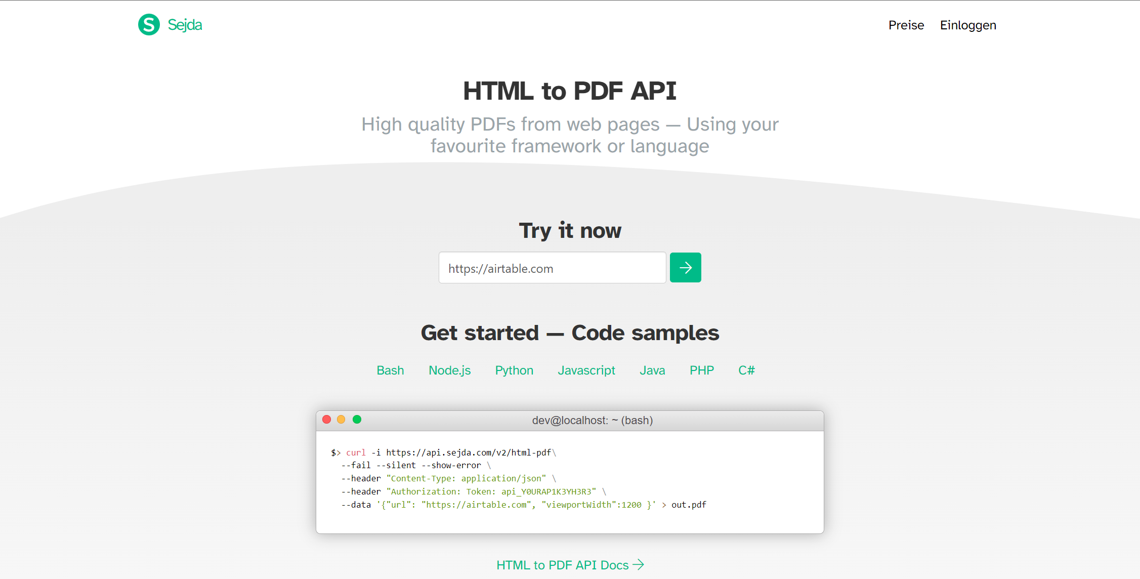
Sejda doe not count the amount of PDFs your generate. You can always create an unlimited amount of PDFs. The only limit by the amount of requests per hour and concurrent requests. We have used the maximum amount of requests allowed per hour to calculate the maximum monthly conversions.
Rate Limit: 4 concurrent requests / up to 48 concurrent requests
Maintainer Remarks:
While the idea of only paying for increased rate limits and concurrency sounds great in general keep in mind that the concurrency limit can limit the overall amount of pdfs you can generate. So while you might be able to generate 216.000 PDFs on the basic plan you will not be able to use that volume when your PDFs take longer to generate.
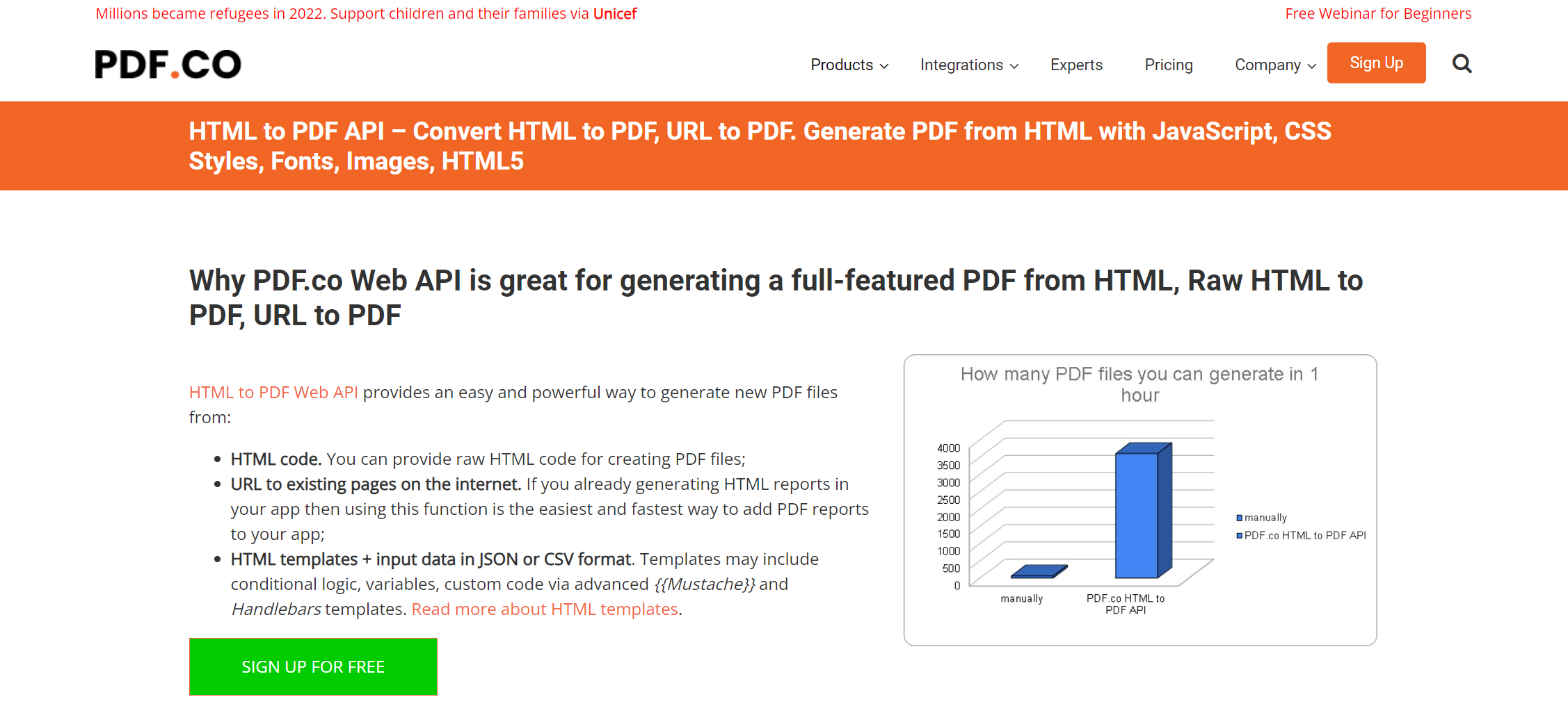
Pricing is based on the amount of PAGES you generate. So if you generate a 10 page PDF you will be charged for 10 pages.
Rate Limit: 2requests per second / up to 25 requests per second
Maintainer Remarks:
PDFco is a service that offers a lot of different PDF related APIs. The HTML to PDF API is just one of them. The pricing is based on the amount of requests you make to all of their APIs. So if you use the HTML to PDF API you can still use the other APIs as well. There also is a credit system that allows you to buy credits and use them for all of their APIs. Credits are used for file uploads and background jobs. I did not include the credit system in the pricing table above since I did not understand it. I guess you will have to contact their support to get more information about it.
Thanks for checking out this front-end coding challenge.
Frontend Mentor challenges help you improve your coding skills by building realistic projects.
To do this challenge, you need a basic understanding of HTML, CSS and JavaScript.
The challenge
Your challenge is to build out this landing page and get it looking as close to the design as possible.
You can use any tools you like to help you complete the challenge. So if you’ve got something you’d like to practice, feel free to give it a go.
Your users should be able to:
View the optimal layout for the site depending on their device’s screen size
See hover states for all interactive elements on the page
Want some support on the challenge? Join our Slack community and ask questions in the #help channel.
Where to find everything
Your task is to build out the project to the designs inside the /design folder. You will find both a mobile and a desktop version of the design.
The designs are in JPG static format. Using JPGs will mean that you’ll need to use your best judgment for styles such as font-size, padding and margin.
If you would like the design files (we provide Sketch & Figma versions) to inspect the design in more detail, you can subscribe as a PRO member.
You will find all the required assets in the /images folder. The assets are already optimized.
There is also a style-guide.md file containing the information you’ll need, such as color palette and fonts.
Building your project
Feel free to use any workflow that you feel comfortable with. Below is a suggested process, but do not feel like you need to follow these steps:
Initialize your project as a public repository on GitHub. Creating a repo will make it easier to share your code with the community if you need help. If you’re not sure how to do this, have a read-through of this Try Git resource.
Configure your repository to publish your code to a web address. This will also be useful if you need some help during a challenge as you can share the URL for your project with your repo URL. There are a number of ways to do this, and we provide some recommendations below.
Look through the designs to start planning out how you’ll tackle the project. This step is crucial to help you think ahead for CSS classes to create reusable styles.
Before adding any styles, structure your content with HTML. Writing your HTML first can help focus your attention on creating well-structured content.
Write out the base styles for your project, including general content styles, such as font-family and font-size.
Start adding styles to the top of the page and work down. Only move on to the next section once you’re happy you’ve completed the area you’re working on.
Deploying your project
As mentioned above, there are many ways to host your project for free. Our recommend hosts are:
We strongly recommend overwriting this README.md with a custom one. We’ve provided a template inside the README-template.md file in this starter code.
The template provides a guide for what to add. A custom README will help you explain your project and reflect on your learnings. Please feel free to edit our template as much as you like.
Once you’ve added your information to the template, delete this file and rename the README-template.md file to README.md. That will make it show up as your repository’s README file.
Remember, if you’re looking for feedback on your solution, be sure to ask questions when submitting it. The more specific and detailed you are with your questions, the higher the chance you’ll get valuable feedback from the community.
Sharing your solution
There are multiple places you can share your solution:
Share your solution page in the #finished-projects channel of the Slack community.
Tweet @frontendmentor and mention @frontendmentor, including the repo and live URLs in the tweet. We’d love to take a look at what you’ve built and help share it around.
Share your solution on other social channels like LinkedIn.
Blog about your experience building your project. Writing about your workflow, technical choices, and talking through your code is a brilliant way to reinforce what you’ve learned. Great platforms to write on are dev.to, Hashnode, and CodeNewbie.
We provide templates to help you share your solution once you’ve submitted it on the platform. Please do edit them and include specific questions when you’re looking for feedback.
The more specific you are with your questions the more likely it is that another member of the community will give you feedback.
Got feedback for us?
We love receiving feedback! We’re always looking to improve our challenges and our platform. So if you have anything you’d like to mention, please email hi[at]frontendmentor[dot]io.
This challenge is completely free. Please share it with anyone who will find it useful for practice.
Fill in the data under columns A to M in the “TITLE LIST” sheet. Based on the data filled in, a code will be generated from a formula in column N.
There is a formula in cell B19 in the sheets titled from “1B. ###” to “13A. ###”, which retrieves the codes from column N in the “TITLE LIST” sheet and automatically fills in the data based on different requirements in each sheet.